Have you ever worked with hierarchical data? I bet you did, even if you don’t know what that means by now. In the context of SQL databases, we define the hierarchical data model as a model in which data are stored as a tree structure, meaning each child record has only one parent. Company role hierarchies, folder structures, and taxonomies (biology) all fulfil this definition. There are a couple of problems the developer needs to solve when working with those data in RDBMS databases. In the past, we were missing built-in tooling in most of the SQL servers for efficient querying of recursive structures that are naturally used to represent those data. What is the situation now in 2024 in PostgreSQL and which models can we use?
The problem and adjacency list
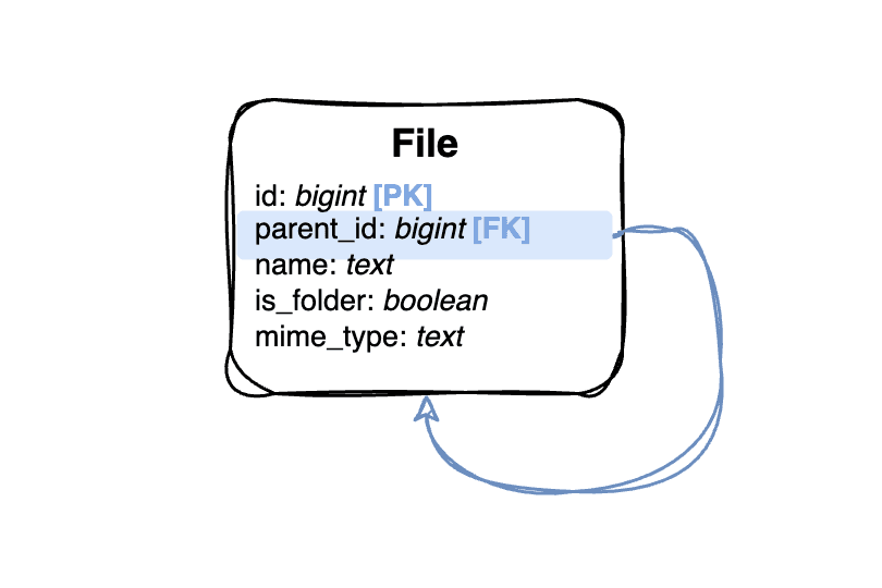
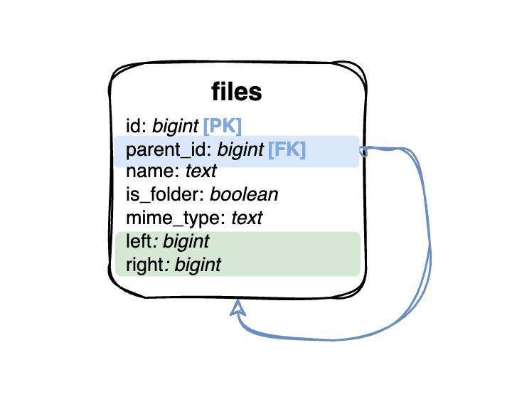
Imagine we have a folder-like structure. We need to store the whole tree with a file name and mime type in a relational database. The first natural opinion for RDBMS modelling is to use a single table with a foreign key referring to itself (parent_id). This simple approach is known as an Adjacency list.
The usage of the adjacency list is very simple. We can add a new file into a folder with a simple database insert, knowing the parent_id. Deleting a whole folder can be achieved using the CASCADE option on the foreign key. Moving a folder into another one can be done with just an update of the parent_id column. The real challenge comes with querying. Showing a single folder content is straightforward with a single where statement, but let’s say we want to have a cool breadcrumb on our website that will show the whole path from a root folder to the file. This means we need to perform a query that will get all of the ancestors of a file with a given ID. With an adjacency list database model, we need to perform a multi-join query based on the number of ancestors the item has. This is where the old database systems reached a limitation because there was no simple way to perform that query with standard SQL. PostgreSQL from version 8.2 has recursive queries that can be used to achieve that. The query for our database model can look like this:
WITH RECURSIVE folders AS (
   SELECT *, 0 AS "depth"
   SELECT *, 0 AS "depth"
       FROM files
       WHERE id = :id
   UNION;
   SELECT parents.*, folders."depth" + 1 AS "depth"
       FROM folders
       JOIN files parents ON (folders.parent_id = parents.id)
) SELECT * FROM folders ORDER BY "depth" DESC;
PostgreSQL will repeatedly replace our search expression in the first union with the new result and make the union of all results in the end. In theory, this still means the database uses multiple join and union operations to retrieve those results. This can be an issue in a large dataset with hundreds of nested rows. PostgreSQL is trying to optimize those queries as much as possible, but there are still more efficient modelling approaches you can take in case the ancestor and descendant (search for all children of file x) queries are your main application usage.
Closure table
When indexing in RDBMS does not provide satisfying results, the mainstream solution nowadays is data duplication. This approach is also possible with hierarchical data modelling. We can create some computed field for each node that will give us all the parents and perform that with a trigger, but the general solution can be achieved with a “closure table”.
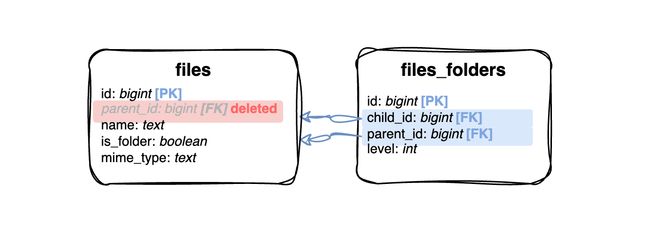
This table should be for all of the relations in the tree graph, including the depth of the relation. We will store not only direct parent-child relations but all of them in one tree. For example, for a file “C” to be in a folder “B” that is located in a folder “A”, we need to store those relations:
| Parent | Child | Depth |
|---|---|---|
| A | A | 0 |
| A | B | 1 |
| A | C | 2 |
| B | B | 0 |
| B | C | 1 |
| C | C | 0 |
You can imagine that the required space to store the closure table will rapidly grow with each additional level of the tree. This also brings a high negative impact on the data modification queries with indexes on foreign keys. The big advantage of this approach is the optimal performance of ancestor, descendant, and level-based queries. The query for our file breadcrumb can look like this:
SELECT folders.*, fc."depth"
FROM files folders
JOIN files_folders fc ON folders.id = fc.parent_id
WHERE fc.child_id = :id
ORDER BY fc."depth" DESC;
Materialized path
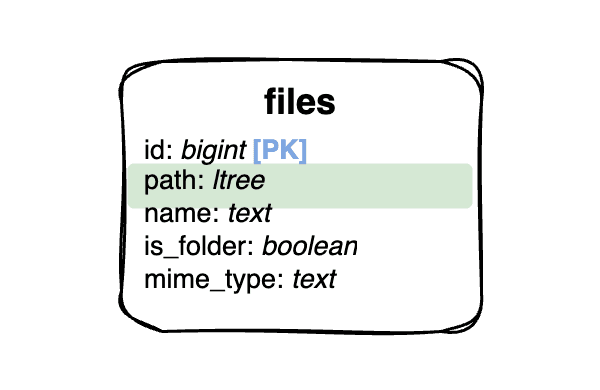
Have you ever worked with cloud file storage providers like Google Storage or AWS S3? Then you probably know that most of them use basic string prefixes to store the information about folders but physically, all of your files are stored at the same place. That’s another modelling approach you can use when working with hierarchical data. Instead of using the foreign key parent_id as in the adjacency list, we will store the string representing the path to this node.
This alone won’t guarantee us any performance improvement over the adjacency list. We need to introduce additional indexing to perform efficient queries. PostgreSQL ltree extension type will help us with that. In addition to good performance, we will also receive additional query power, which is not limited only to ancestors and descendants using the lquery. Let’s take a look at the lquery for our breadcrumb:
SELECT * FROM files WHERE path @> (
   SELECT path FROM file WHERE id = :id
) ORDER BY path;
This looks elegant, but the main issue with this modelling in PostgreSQL is that the GIST index used for the ltree requires size limitation, so we can’t use it for really nested trees. The movement of one subtree into another is also more complex since we need to update all the inside of the folder.
Nested set and intervals
The last approach that we should discuss is the nested set model. It is based on the tree traversal principle. We start at the root node of the tree and go to the leftmost leaf node. Once we reach it, we go back until we reach a node that has multiple children, go into the next unvisited leftmost child, and repeat the process until we visit all of the nodes. Let’s count all visits of the nodes in the tree in each node store this count two times:
- Left: The count when we visit the node for the first time (going down)
- Right: The count when we visit the node for the last time (going up)
This process is shown in the image below.
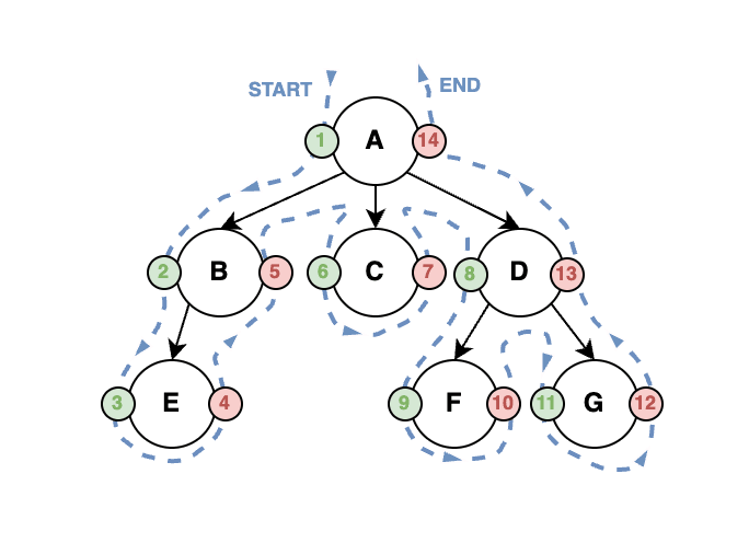
These numbers can be used to very efficiently perform descendant and ancestor queries without increasing the database size drastically. We just need to know the left and right values.
// Descendants
SELECT * FROM files WHERE
"left" > :left AND WHERE "right" < :right
// Ancestors
SELECT * FROM files WHERE
"left" < :left AND "right" > :right
This solution assumes we have only one tree in our database. We can also store an ID of the root node in all children to make sure we take nodes only from the right tree. This field can also be helpful in different queries (e.g. find the root of the current node).
We achieved very good ancestors performance, but we lost the options to query direct ancestors and direct descendants, meaning we have a fast breadcrumb, but we are not able to simply show the contents of a single folder. We also increased the complexity of insert, delete, and move operations because we need to recalculate all the right and left numbers in the right subtrees of the same tree. This operation can be expensive, but there are some ways how to recalculate all the values pretty fast, some of them are mentioned in the blog Hierarchies on Steroids #1 by Jeff Moden.
The solution for the modification queries is the use of intervals instead of integers for left and right values. We can simply insert the node into the subtree using decimals. The straightforward solution using halving the left and right values can fail very quickly and hard on decimal precision, that’s why there are multiple approaches how to encode the nested intervals. If you are curious about some of the basic methods, I can recommend reading Nested Intervals Tree Encoding in SQL by Vadim Tropashko.
Summary
There are multiple ways of hierarchical data modelling in SQL. PostgreSQL has good support for most of them. A good recommendation is to always start with the adjacency list solution since it is simple, space-efficient and can be easily combined with any other solution mentioned above. The closure table and materialized path solutions offer good performance and also additional usage with more than just ancestors and descendant queries, but those are just benefits you will pay with limitations of the tree size.
If you have trouble querying your large hierarchical dataset with deep subtrees for descendants and ancestors, always remember nested set and nested interval solutions. We can use them just as an index for querying since the space requirements are equivalent to the adjacency list solution and we can rebuild them quickly. Adjacency list can take the rest of the job for you.